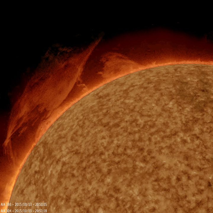
In the Project Hail Mary movie there are cells that come from the surface of the Sun. This is the long version of where that idea took me, from what life would need there to the two plasma simulations I ran and why I stopped, with the numbers.
In Project Hail Mary there are these cells called Astrophage, and they come from the surface of the Sun. So, lifeforms living on the surface of the Sun. I stopped watching as soon as they said that and went off with my own idea, before the movie even got to showing that the cells were made of carbon, hydrogen and oxygen. I only found that part out later. But if something actually wanted to survive on the surface of the Sun, it would probably have to be made of the stellar plasma too.
Plasma is gas in which enough electrons have come loose from their atoms that the whole thing conducts electricity, so it drags magnetic field around with it and the field pushes back. The outer layers of a star are made of it. The Sun's visible surface is only weakly ionized, and cool enough that a few molecules form there, but it gets hotter and more fully ionized higher up. A lifeform living in those layers wouldn't get much choice of material, and hot magnetized plasma is the obvious candidate.
Plasma life on its own isn't a new idea. Tsytovich and others suggested back in 2007 that helical structures of charged dust grains in cold, dusty plasma could behave a bit like living matter.1Tsytovich et al. (2007), New J. Phys. 9, 263. Their structures are built from charged solid microparticles, so the grains are part of the idea. Reference. The surface of a star is a very different place, dust grains wouldn't survive there, so I was asking about the hot magnetized plasma itself.
That's way too big a question to simulate, so I asked a smaller one: if you write a pattern into plasma, can you read it back later?
I ran two tests. In the first, a magnetic wave written into a box of moving plasma could still partly be read at the end, but by then the electrical resistance I had chosen would have shrunk it to about a tenth of its starting size even with nothing else going on, so how much of it survived mostly depends on one setting I picked. The second wrote a heat pattern near a point where the magnetic field is zero and tried to read it by pushing on the plasma, and the reading changed so much on a finer grid that it failed the check I had fixed in advance in all eight cases. It can't say whether the pattern was read or lost. I came out of it with a sharper version of the question and a list of what a test would need to answer it.
What life needs without water and carbon
The first thing was working out what life actually needs once you take away water and carbon. Water and carbon are parochial requirements, which means they're just how life happens to work on Earth. Pattern is different. If something has no structure you can tell apart from its surroundings, you can't even say it's there, never mind alive.
The pattern doesn't have to keep the same material, though. A flame is always burning new fuel and it's still one flame. A hurricane keeps pulling in new air and throwing old air out, and it's the same hurricane from one day to the next. The useful question for a plasma lifeform is then what it would have to keep, whatever it happens to be made of at the moment.
The reason pattern matters is lineage: a parent has to pass something on to whatever comes after it, and that something is a pattern. For us that's DNA and RNA, where the order of the bases is what gets copied. A plasma lifeform would need its own version of that.
That rules out the cheapest version of plasma life. Structures form in a star's atmosphere all the time and fall apart again, and if one forms, dissolves, and a similar one shows up later on its own, the second one didn't inherit anything from the first. I'll call that recurrence, and snowflakes and ripple marks in sand recur constantly without anyone calling them alive. To count as a lineage, the first structure has to leave something behind that changes what forms next, some trace in the field or the gas that the next one picks up.
So the question turned into one about information: can a plasma hold a pattern for long enough, and can you read it back later?2Scharf and Witkowski (2024) rebuild the habitable zone from the bottom up around computation, meaning physical processes that act on information stored in states of matter, and call the result computational zones. My question sits inside that idea, for one very hot environment. Reference.
A first draft that didn't survive
Every time I tried to argue that plasma life was impossible, the argument turned into a question about some quantity I could actually calculate. So I wrote it all down.
A good chunk of that first document didn't survive checking. I had claimed chemistry fails completely in the Sun's photosphere, but molecules like CO do form there.3Carbon monoxide has been observed in the solar atmosphere for decades, and Wedemeyer-Böhm and Steffen (2007) model it forming and breaking apart in the photosphere and chromosphere. Reference. A couple of other arguments, like a hard limit on how many magnetic structures could exist side by side, needed assumptions I hadn't justified.4That limit leaned on magnetic helicity, a measure of how twisted and linked a field is. Two closed flux tubes that aren't linked have zero mutual helicity no matter how close together they are (Démoulin, Pariat and Berger 2006), so crowding structures together doesn't set a limit on its own. Reference.
The part that held up was the framing. Life needs a lineage, a lineage needs a pattern that gets passed on, so the question is how long a turbulent magnetized plasma can remember a pattern and whether anything can read it back.
Before simulating anything I needed a definition of remembering, and the one I used is plain. Write one of two possible patterns into the plasma, wait, and then check whether some reader can still tell which one you wrote. If it can't do better than a coin flip, the plasma has forgotten, at least as far as that reader is concerned. One bit is a small message, but it's enough to see whether anything survives at all.
Test one: a wave in the field
The first test wrote magnetic patterns into a simplified plasma simulation, as one of two signs of a chosen wave pattern, and checked whether a reader could still tell which sign it was later. With the right reader, some of it stayed readable.
The simulation was a periodic box, a cube 2π on a side with 24 grid points each way, filled with an incompressible magnetized fluid that has some electrical resistance. The message was a magnetic wave added to a random moving background, with either a plus or a minus sign in front of it. After the plasma had evolved for a while, the reader projected the field back onto the wave, got a number, added its own measurement noise, and guessed the sign from whether the number came out positive or negative. The noise was Gaussian with a fixed size σ, in units where the wave starts with a mean square of 1, and I tried σ = 0.1, 0.3 and 1. I ran this on 32 different random backgrounds, both signs on each, so 64 runs. Everything is in simulation units, so the box isn't tied to any particular place on the Sun.
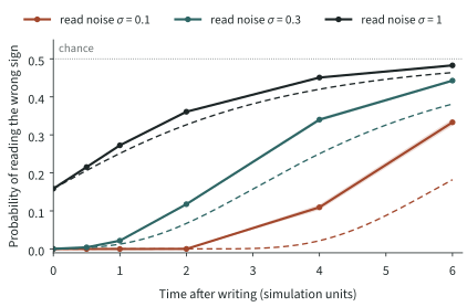
By t = 6 in simulation units, the least noisy reader got the sign wrong 33% of the time (Figure 1). That 33% is a probability: for each run I worked out the chance of a wrong guess exactly from the noise, then averaged over the 64 runs. A coin gets it wrong 50% of the time, so part of the bit was still there, about 0.08 bits. The bits are the mutual information between the sign I wrote and the reader's guess, which is 1 bit for a reader that's never wrong and 0 for one that's wrong half the time. The same reader on the wave alone, with no background and nothing happening except the wave slowly fading, gets it wrong 18% of the time. The moving background made it worse, which is about what you'd expect, but it didn't wipe the message out.
Most of the fading comes from the resistance. On its own the wave decays by diffusion as , and with the diffusivity η = 0.1 I chose and the wave's wavenumber k = 2 that is e−2.4 by t = 6, about 9% of its starting size. So how much of the bit survives here is mostly set by the value of η I picked, and the background accounts for the step from 18% to 33%.
That reader was generous though. It knew exactly where the pattern was supposed to be, and it got to look at the whole simulation at once.
The first of those matters because, for a single wave on its own, sliding it by half a wavelength is the same as flipping its sign, so if the reader doesn't know where the wave starts, a plus and a minus look identical and the message is gone. I tried a second code that carries its own reference, a longer wave written alongside the message wave, so the reader compares the two waves with each other and doesn't need to know where anything is. That kept some of the bit too. Its least noisy reader was wrong 37% of the time, against 29% for the same code with no background.5The two codes aren't a fair race. They use different observations and split the signal energy differently, so each one is compared with its own no-background case. But it's still a reader looking at the whole box from outside, and nothing in the plasma was doing any reading.
Test two: heat near a magnetic null
So the second test was local. Near a magnetic null, where the field drops to zero, I heated the plasma in one of two patterns with the same total energy, then pushed on the middle later and watched how the plasma nearby moved.
I picked a null because one kick is enough to keep it changing for a while. In this setup the field starts in an X shape, with field lines bending away from a point in the middle where the field is zero. A disturbance comes in from outside and collapses that X into a thin sheet of electric current, and the current in the middle then flips sign back and forth as it dies down.6The setup is informed by work on oscillatory reconnection, for example Karampelas et al. (2022), who found that the period of these oscillations doesn't depend on how strong the initial pulse is. My transport settings were chosen to make a local test tractable, so this isn't a calibrated model of the solar corona. Reference. That flipping is a small, simple version of a structure that comes back more than once, and a lineage would need something like that, something that returns and could carry a pattern from one round to the next. The plan was to write the pattern before the current flipped and read it after. Nulls like this are usually studied in the corona, the hot thin layer well above the visible surface, so this test had moved up from the surface I started with, and like the first one it's in simulation units.
The writing was heat. Between t = 2 and 2.2 I added heat in a ring around the null, and the ring was either hotter along the x axis or hotter along the y axis, with the same total energy either way (Figure 2). I'll call these the cosine patterns, because the heating varies around the ring as cos 2θ. At its strongest the added heat was about 12% of the internal energy already there in the runs with the incoming disturbance, which had squeezed the plasma in some parts of the ring and thinned it in others by then, and about 10% in the runs without it. A second pair, the sine patterns, did the same thing rotated by 45 degrees. The field doesn't look the same after that turn, though. The sine patterns put their hot spots on the diagonals, which are the two field lines that run through the null, and their readers (below) sat closer to it, so the two pairs aren't exact copies of each other.
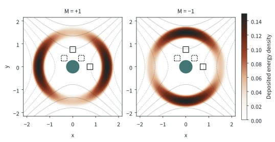
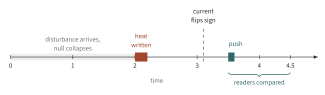
Then I waited. The central current flipped at about t = 3.1, and at t = 3.5 I gave the plasma a short, small inward push inside a small disk at the centre, lasting 0.1 time units. Four small square readers nearby averaged the velocity of the plasma inside them for the next time unit (Figure 3). Two sat on the x and y axes, 0.75 from the null, and were read for the cosine patterns. The other two sat on the diagonals, about 0.53 from the null, and were read for the sine patterns.
The reading needs one more step, because a push makes the plasma move whether or not there's a pattern. For each pattern I ran the simulation twice from the moment before the push, once with the push and once without, and took the difference, which leaves only what the push did. Then I compared that between the two patterns. If the heat pattern changed how the plasma answers the push, this is where it shows up.
The push is there because of the lineage idea from earlier. A pattern only matters for a lineage if it changes what the plasma does next, and the push response asks whether the heat changed how the plasma moves. Reading the temperature directly would only show that the heat is still there. It is still a reader from outside, though, since I chose the push, when it came and where the readers sat.
There were eight cases: two values of the heat conductivity κ, 0.2 and 2.6 (the heat flows mainly along the field lines, except near the null where the field is weak), the two orientations of the pattern, and runs with and without the incoming disturbance. The runs without it are a control. The heat can still make the plasma move and the field change on its own there, and I wanted to know how much of any response needed the flipping current.
There is no read noise in this test, so the coin flip from the definition becomes a question about numerical error. Before running anything I had set a rule that the effect had to be clearly bigger than the numerical noise, five times bigger in the version I wrote down, and if it isn't, this reader can't tell the two patterns apart. Passing that rule was the condition for the big campaign, which meant running the same test with many more disturbances. One part of that noise is easy to measure, so it was the first thing I checked.
Doubling the grid
A simulation chops the plasma into grid cells, and the answer can depend on how small the cells are. The physics doesn't know how many cells you used, so the usual check is to run the same thing again on a finer grid, where a real effect should come out about the same. I ran everything at 160 cells per side and again at 320.
The heat patterns were mostly still there, but when I doubled the grid resolution the readout changed, and in some cases it flipped sign (Figure 4). A real signal shouldn't change like that when you only change the resolution.
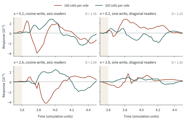
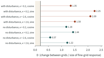
To put a number on it I took the difference between the two grids' response curves and divided it by the size of the fine-grid response, and I call that ratio D. For the readout to count, D had to be under 0.2. The eight cases came out between 0.57 and 2.25 (Figure 5), so in the best case the grid changed the answer by more than half its own size, and in the worst case the change was more than twice the answer.
In three of the four runs with the disturbance, the average response over the reading window has opposite signs on the two grids. In one of them the size of the response changed by only 12%, from 1.60 to 1.40 millionths of a velocity unit, while its shape changed completely, so looking at the size alone would have been a little too reassuring. Percentage changes in the text are relative to the coarse-grid value, while D divides by the fine-grid one.
The flip itself moved with the grid too. On the finer grid the current flipped about 0.1 time units later, while the push stayed at t = 3.5 (Figure 3). I compared the curves at the same clock times without shifting them to line up, as decided before the runs, so part of the mismatch could come from this timing shift. I didn't check how much.
The control runs made it harder still. The runs without the incoming disturbance respond to the heat pattern too, and their responses are about 10 to 30 times larger than the ones with it. A response to the heat doesn't need the flipping current at all, then, and comparing the two families doesn't isolate the current as the cause. The grid dependence also means this readout can't be used as evidence that the plasma erased the message, or that it kept it.
What did survive
The heat patterns themselves were still distinguishable later, and at low conductivity they only changed by 6 to 8% between resolutions. At t = 4.5, which is 2.3 time units after the heating stopped, in the runs with the disturbance and no push, half the temperature difference between the two cosine patterns at the axis reader was 0.003035 on the coarse grid and 0.002787 on the fine one, in units where the starting temperature is 1.
Higher conductivity spreads heat along the field faster, and there it was worse. The same temperature difference changed by about 47% between grids. I also measured an entropy, ln(p/ργ) from the pressure p and density ρ, which unlike temperature doesn't change when a piece of plasma is squeezed without being heated, and its much smaller difference for the rotated pattern flipped sign, from 2.0 × 10⁻⁶ to −2.9 × 10⁻⁶.
A written heat pattern does stay around near the null for a couple of time units in this model. That counts for something, but nothing in the simulation reads it. These differences are measured at fixed places in the grid, and the plasma flows through those places, so they don't follow any particular piece of plasma and they don't show anything being carried from one flip of the current to the next. Heat lingering near a null after heating stops has also been studied properly before, by Johnson and colleagues (2024) and Cargill and colleagues (2025) among others, so on its own it wouldn't be new.7Both are papers in Monthly Notices of the Royal Astronomical Society on heating and cooling at coronal magnetic nulls. References: Johnson 2024, Cargill 2025.
Why I stopped
So I held off on the big campaign. Running many more copies of a readout that depends on the grid wouldn't have told me anything new.
Part of the problem was the push itself. At 160 cells per side the push region covered 16 cells and at 320 it covered 76, and the strongest velocity it gave the plasma rose from 0.00306 to 0.00359 even though the push was set to the same strength on both grids. The reader squares were 0.25 wide, two cells across on the coarse grid. The response also wasn't cleanly proportional to the push. Halving the push changed the rescaled response by 13 to 29%, so I couldn't treat it as a gentle probe that just reads what's already there.
The obvious fix was another doubling, to 640 cells per side. A short timing test at the higher conductivity took 147 seconds to get to t = 0.02, which works out to about nine hours for the reference run from the start to t = 4.5 at that conductivity, and I had given each run two hours, which was a little short, by a factor of four and a half. That's just the reference run the written runs start from, before any of the eight cases and their branches, so it wasn't going to happen with this code on my laptop.
For physicists: setup, rule and numbers
Everything is in dimensionless simulation units. No stellar location or physical lifetime is inferred from either test.
Test one: Fourier memory in a periodic box
Incompressible resistive MHD in a periodic cube of side 2π, 243 grid, viscosity and magnetic diffusivity both 0.1, field in Alfvén-speed units. An unbiased message M = ±1 is written as with carrier (unit mean square). The background excludes the carrier Fourier pair, so the two writes start with matched energy and helicity. Background velocity and magnetic rms are 0.5 each. The reader knows the carrier's position and orientation, projects onto and adds Gaussian noise of fixed σ. With no background the solution is exact, and , so the optimal error is . At t = 6, ηk2t = 2.4 and diffusion alone leaves e−2.4 ≈ 0.091 of the carrier amplitude. The error is the probability of a wrong sign, integrated exactly over read noise for each run and averaged over the 32 background pairs (64 runs). Results at t = 6:
| σ | error (95% interval) | pure diffusion | information (bits) |
|---|---|---|---|
| 0.1 | 0.3331 (0.3243–0.3419) | 0.1822 | 0.08193 |
| 0.3 | 0.4427 (0.4395–0.4459) | 0.3812 | 0.00950 |
| 1.0 | 0.4827 (0.4818–0.4837) | 0.4639 | 0.00086 |
The information column is the mutual information between M and the reader's sign guess, pooled over all runs, which is 1 − H2(p) for error p and binary entropy H2. It is not the channel capacity. The internal-reference code writes a k = 1 reference and a k = 2 target with half the signal energy each and reads the translation-invariant . At σ = 0.1 its error is 0.3737 (0.3680–0.3796) against 0.2901 for its own pure-diffusion reference, with 0.04652 bits. Representative 24 versus 32 grid and half-timestep checks passed an absolute read-error tolerance of 0.001, with the largest grid change about 5 × 10⁻⁶.
Test two: a local heat write near an X-point
Two-dimensional compressible resistive MHD on x, y ∈ [−10, 10], initial B = (y, x), ρ = p = 1, γ = 5/3, T = p/ρ, magnetic diffusivity η = 0.04, with a divergence-preserving magnetic update. Heat conduction is anisotropic, with κ = 0.2 or 2.6 and Biso = 0.2, so it becomes isotropic at the null. The disturbance is an initial velocity ring, v = w(r) (x, −y)/r2 with , peak speed about 0.4 near r = 5. Walls are stationary, impermeable and conducting, held at T = 1. To absorb the outgoing wave, the velocity at r ≥ 7 is set to zero once at t = 0.6 (its kinetic energy is recorded), and after t = 0.6 a velocity damping rate 1 + tanh(r − 5) and a kinematic viscosity 0.1[1 + tanh(r − 5)] act at r ≥ 3, with both zero closer to the null. In the runs with the disturbance the null current is negative at t = 2 and first crosses zero at t = 3.06 (κ = 0.2) and 3.09 (κ = 2.6) with 160 cells per side, and at 3.16 and 3.20 with 320. The control runs remove the disturbance and still solve full MHD.
The write acts from t = 2 to 2.2 with deposited internal energy density
zero outside 1.15 < r < 1.85, and sin 2θ for the rotated orientation. Total deposited heat is 0.397375 at N = 160 and 0.398179 at N = 320 per unit length. The peak is about 12% of the local internal energy just before writing in the disturbance runs and about 10% in the controls, where the internal energy is still close to its initial p/(γ − 1) = 1.5. The probe is an inward radial acceleration supported in r < 0.3 from t = 3.5 to 3.6 with integrated coefficient A = 0.01. Readers are squares of side 0.25 centred at (0.75, 0) and (0, 0.75) for the axis channel and (±0.375, 0.375) for the diagonal channel, fixed in physical space under refinement. The axis observation Y is mean vx at the x reader minus mean vy at the y reader, and the diagonal observation is the difference of the two outward diagonal velocities. Cosine writes use the axis channel and sine writes the diagonal one. The diagonal readers sit at r ≈ 0.53 on the initial separatrices y = ±x and the axis readers at r = 0.75, so the two orientations are not equivalent under a 45 degree rotation. The measured response contrast (R for response) is
on common times from 3.5 to 4.5, with norm by the trapezoidal rule and no phase alignment.
The rule fixed before the written runs required the effect to exceed five times its numerical uncertainty, taken as the largest discrepancy among grid refinement, half timestep, domain size and a zero-write null. The grid discrepancy is one of those, so on its own it already requires
| Runs | κ | write | rms, N = 160 | rms, N = 320 | D | mean sign |
|---|---|---|---|---|---|---|
| disturbance | 0.2 | cosine | 1.602 × 10⁻⁶ | 1.403 × 10⁻⁶ | 1.348 | − / + |
| disturbance | 0.2 | sine | 1.283 × 10⁻⁶ | 8.158 × 10⁻⁷ | 2.252 | + / − |
| disturbance | 2.6 | cosine | 1.614 × 10⁻⁶ | 1.324 × 10⁻⁶ | 2.091 | − / + |
| disturbance | 2.6 | sine | 6.628 × 10⁻⁷ | 4.519 × 10⁻⁷ | 1.503 | + / + |
| control | 0.2 | cosine | 2.293 × 10⁻⁵ | 1.511 × 10⁻⁵ | 1.180 | − / − |
| control | 0.2 | sine | 1.729 × 10⁻⁵ | 1.215 × 10⁻⁵ | 1.436 | + / + |
| control | 2.6 | cosine | 1.464 × 10⁻⁵ | 1.419 × 10⁻⁵ | 0.569 | − / − |
| control | 2.6 | sine | 1.230 × 10⁻⁵ | 1.303 × 10⁻⁵ | 1.217 | + / + |
RMS values are in simulation velocity units over the full window. Mean sign is the sign of the time-averaged CR at N = 160 and N = 320.
All eight cases fail. The probe itself is under-resolved: it has 16 nonzero cell-centre samples at N = 160 and 76 at N = 320, and its sampled peak velocity increment rises from 0.003060 to 0.003585 at fixed A. On the coarse grid, ‖2C(A/2) − C(A)‖/‖C(A)‖ is 16.6%, 13.3%, 27.0% and 29.2% for κ = 0.2 cosine and sine, then κ = 2.6 cosine and sine.
Thermal states survive better. Half the difference between patterns at t = 4.5 in the no-probe disturbance runs, at the x-axis reader for cosine and the positive diagonal reader for sine, with temperature averaged cell by cell and the entropy proxy ln(p/ργ):
| κ, write | T, N = 160 | T, N = 320 | entropy proxy, N = 320 |
|---|---|---|---|
| 0.2, cosine | 0.003035 | 0.002787 | 0.004149 |
| 0.2, sine | 0.0007448 | 0.0007862 | 0.00116 |
| 2.6, cosine | 0.0005085 | 0.0007457 | 0.00131 |
| 2.6, sine | 0.00006091 | 0.00006837 | −0.000002921 |
For κ = 2.6 sine the entropy proxy at N = 160 is +2.00 × 10⁻⁶, so it reverses sign under refinement while the temperature contrast does not. Compression can contribute to a local temperature difference.
Independent checks and cost
An independent Athena++ implementation (Stone et al. 2020) passed basic wave checks and no-conduction X-point energy bookkeeping at N = 256 and 512, closing to about 10−12. That checks the MHD integration without heat conduction only. It cannot check the thermal experiment, because the anisotropic-conduction routine in the Athena++ version I used is empty. Three separately written analyses of the raw fields and a direct reconstruction give the same eight D values to the digits in the table, and two of them match on the eight fine-grid response norms to within 9 × 10⁻¹⁹ in velocity units. An isolated N = 640, κ = 2.6 timing test completed 180 steps to t = 0.02 in 147.39 seconds of solver time. Combined with the explicit thermal timestep limit this gives about nine hours to t = 4.5, an early-time extrapolation, against a cap of two hours per run.
What the numbers do not show
The subtraction uses a matched no-probe history that a reader given one unknown message would not have. Comparing background families does not isolate reconnection as the cause. Thermal persistence at fixed points is not a decoder and does not identify anything carrying the pattern through cycles. None of this sets a universal limit on plasma life or a stellar habitability boundary.
What a better setup needs
Any result, either way, needs a readout that converges first. If a written pattern can be read near a recurring structure and the readout stays the same when the grid is refined, it's worth running in bulk and testing against controls. If it converges and turns out to be fully explained by ordinary heat transport and flow, then this route doesn't work, at least in this form. Right now it's neither, and the next version would need a few things this one didn't have.
- One local quantity, read with a protocol written down in advance, that passes the grid and time-step checks before anything gets run in bulk.
- A reader that works from a single run. My subtraction used a matching unpushed run for each pattern, and a real reader holding one unknown message wouldn't have that, so either the reader manages without it or the calibration becomes part of the setup.
- A control that changes one thing. Taking out the disturbance changed the heat, the flows and the field history all at once. A better control keeps the same thermal and flow background and switches off only the magnetic process being tested.
- A faster or different solver. A full reference run at 640 cells per side and the higher conductivity didn't fit the time I had, and the version of the independent code I used as a check had no working anisotropic heat conduction.
- Further out, a recipient. Something that starts out independent would have to pick up the pattern through the plasma's own fields and still have it after they separate, with the copying coming out of the physics and no copy rule put in by hand.
I've stopped working on it for now, but none of this means plasma life is impossible, and I might come back to it with a better setup.
References
Cargill, P. J., Hood, A. W., and Johnson, D. 2025, Heating and cooling at a coronal magnetic null, Monthly Notices of the Royal Astronomical Society 542, 3385–3394. doi:10.1093/mnras/staf1444
Démoulin, P., Pariat, E., and Berger, M. A. 2006, Basic properties of mutual magnetic helicity, Solar Physics 233, 3–27. doi:10.1007/s11207-006-0010-z
Johnson, D., Hood, A. W., Cargill, P. J., Reid, J., and Johnston, C. D. 2024, The thermodynamic response of heating at coronal null points, Monthly Notices of the Royal Astronomical Society 532, 4261–4271. doi:10.1093/mnras/stae1760
Karampelas, K., McLaughlin, J. A., Botha, G. J. J., and Régnier, S. 2022, The independence of oscillatory reconnection periodicity from the initial pulse, The Astrophysical Journal 933, 142. doi:10.3847/1538-4357/ac746a
Scharf, C., and Witkowski, O. 2024, Rebuilding the habitable zone from the bottom up with computational zones, Astrobiology 24, 613–627. doi:10.1089/ast.2023.0035
Stone, J. M., Tomida, K., White, C. J., and Felker, K. G. 2020, The Athena++ adaptive mesh refinement framework: design and magnetohydrodynamic solvers, The Astrophysical Journal Supplement Series 249, 4. doi:10.3847/1538-4365/ab929b
Tsytovich, V. N., Morfill, G. E., Fortov, V. E., Gusein-Zade, N. G., Klumov, B. A., and Vladimirov, S. V. 2007, From plasma crystals and helical structures towards inorganic living matter, New Journal of Physics 9, 263. doi:10.1088/1367-2630/9/8/263
Wedemeyer-Böhm, S., and Steffen, M. 2007, Carbon monoxide in the solar atmosphere. II. Radiative cooling by CO lines, Astronomy & Astrophysics 462, L31–L35. doi:10.1051/0004-6361:20066173
Figures 1, 4 and 5 are redrawn from the saved outputs of the runs. Figure 2 shows the prescribed heat source and Figure 3 is a schematic.